Now imagine in the 1960’s Fred’s idea of the continuous arrival of new matter arriving in our visible universe, at exactly the rate required to balance the observed expansion.
What would that universe look like?
This is the view Rourke provides. He uses de Sitter Space, in which pairs of geodesics eventually separate exponentially, in both forwards and backwards time.
It is a natural first model for a universe, one with constant curvature. New galaxies are constantly arriving in our backwards light cone, and do so highly redshifted as gamma-ray bursts. It is not new matter, spontaneously created, it has existed a very long time, but has only just now entered our visible universe. We will see it until the end of time.
What if the waves we are seeing are not drammatic in-spirals of black holes, but are the result of the same modulation of gravitational waves generated by the central black holes of galaxies?
Earlier in the year I submitted a proposal to this conference in Glasgow about general relativity and gravitational waves birch.
Is there anything else? Colin Rourke, on light.
The CMB and gravitational waves should be in equilibrium due to the Rees-Sciama effect?
After submitting the talk, I realised the subject was a little more complex than I had hoped, requiring not just de Sitter Space, but also the model of galaxy evolution outlined in Rourke’s work, where galaxies are characterised by the size of their central black holes.
The release of data from the Dark Energy Spectroscopic Instrument has provided ideal data to help determine the split between cosmological and intrinsic redshift.
The key idea is that smaller black holes exhibit intrinsic redshift, with light coming from close to the black hole. As the central black hole and galaxy grow the redshift diminishes and is negligble in a full size galaxy.
The talk was not accepted, which was somewhat of a relief. It has taken me some time to understand what is going on with galaxy spectra.
I had also made the submission before I heard the very sad news that Colin Rourke had passed away.
I decided I would still attend the conference, as it gave an ideal opportunity to get the latest information on gravitational wave observations and next generation detectors. I was not disappointed.
Is the green valley a rainbow mountain in disguise?
There’s a hill with a green chair, lined by birch, a green valley, if you will.
It’s a place I have spent much time musing about space and time.
This module is about a new mountain, where the jackets are all colours of the rainbow.
It asks if there is in fact no valley at all, but an illusion of such due to the assumption that redshift and distance follow an exact Hubble law.
The *green valley* is a wide region separating the blue and red
peaks in the ultraviolet optical color magnitude diagram, first
revealed using GALEX UV photometry.
This is how the green valley galaxies are described by the 2014 paper of Samir Salim: https://arxiv.org/pdf/1501.01963
Here is an image and caption from the paper:
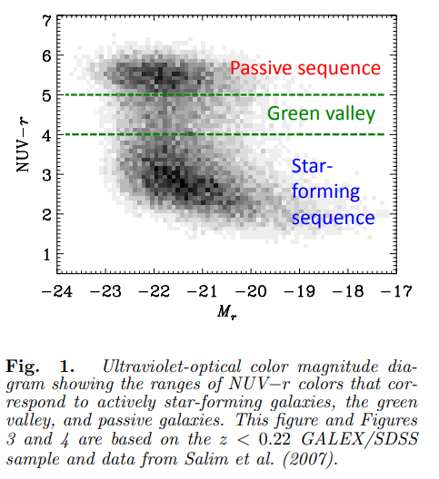
It is based on observations of distant galaxies in the ultra-violet spectrum, specifically what is referred to as the NUV-r range.
NUV stands for Near Ultraviolet and -r, I presume, is an indication that the frequencies have been shifted to make it look like the familiar red to blue frequency range in light. update: it appears in the literature that NUV-r is taken as a good indicator of star formation rate.
In effect, the telescopes making the observations are taking the temperature of the galaxy being observed, the hotter it is, the bluer the result.
It is also possible to measure the red-shift, with good precision, of each galaxy that is observed.
Assuming an exact Hubble law, we can translate redshift into distance.
If it is also assumed that there was a big bang, redshift is used to estimate the age of the galaxy.
Once we have the distance, we can translate the apparent magnitude into an absolute magnitude.
Combining this with the age of the galaxy we get an estimate of star formation rate.
The curious observation is that across a wide range of magnitudes we see many red galaxies and many blue galaxies, but far fewer in the green region, a green valley if you will.
The conclusion is that there are two classes of galaxies. Ones that are actively forming stars and ones that are less active in forming stars. It is also assumed the transition from active to quiescent galaxies happens rapidly, hence we see fewer galaxies in this stage.
Explaining the Green Valley
What if the relationship between redshift and distance is not in fact exact?
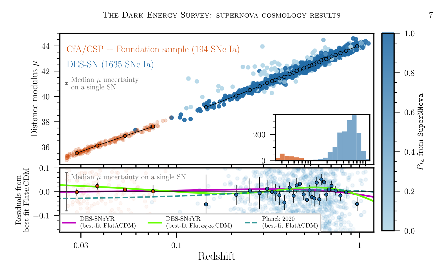
There is good evidence for this from the Dark Energy Survey, based on observations of supernovae, that the relation is not exact.
This is a central theme of The Geometry of the Universe. de Sitter Space, a uniformly, curved space-time, is suggested as a good model for what we see.
In de Sitter Space, the Hubble law only holds asymptotically.
There are galaxies both sides of the asymptote. Here is an image that attempts to show the relationship:
The image was created using the Spiral Galaxies, no dark matter module, simulating many random galaxies arriving in our visible universe, noting the redshift and distance of the galaxy as it steps through our time.
At any particular redshift we see galaxies over a wide range of distances. For galaxies with no redshift (z=0) it turns out that they are most likely to be at 2/3 of the Hubble distance.
de Sitter Space is a space-time which has the Perfect Copernican Principle: there are no special places or times in the universe.
In such a universe, there is no overall expansion. It exhibits red shift, but also blue shift in the form of gamma-ray bursts, galaxies arriving at the edge our visible universe.
There is an asymptotic relationship between z and d, both in forwards and backwards time.
Closer to home, there are galaxies bursting on the scene, at z=1. Half immediately recede, the other half zoom closer. All eventually converge to the Hubble-law asymptote.
The Green Mountain
Now imagine what happens if this is what we are observing, but we assume an exact Hubble law to gauge distance and size.
If a galaxy turns out to be nearer than the Hubble law would imply, we end up over-estimating it’s magnitude, since the object we are seeing is nearer than we think.
If a galaxy is further away than the Hubble law implies, we under-estimate it’s size.
The set of galaxies that are observed varies over 7 magnitudes, with z < 0.22.
Our sample of galaxies that are further away than we are assuming will be a sample of large galaxies, that we mistakenly assume are small.
The sample of galaxies that are nearer than we are assuming, will be a sample of small galaxies that we are assuming to be large.
The galaxy model in the Geometry of the Universe also proposes a quasar-galaxy spectrum, in which small quasars grow into large galaxies over a long period of time. It suggests there is a general evolution as the central black hole grows in size.
In the image of the green valley, the passive sequence includes galaxies whose size has been underestimated, they will move to the left in the image.
The star forming sequence includes galaxies who’s size has been over-estimated. Correcting this will move them to the right in the picture.
The end result? There is still a green valley.
I should add there is a good way to test this theory. The supernovae data, from the dark energy feature a growing set of galaxies for which we have good evidence their true distance: supernovae have very consistent brightness.
I wonder what the colour-magnitude diagram for this set of galaxies looks like? My guess is that most supernovae we see are associated with large galaxies and will likely be in the green valley.
And how to show this in code?
Update 2025/1/25
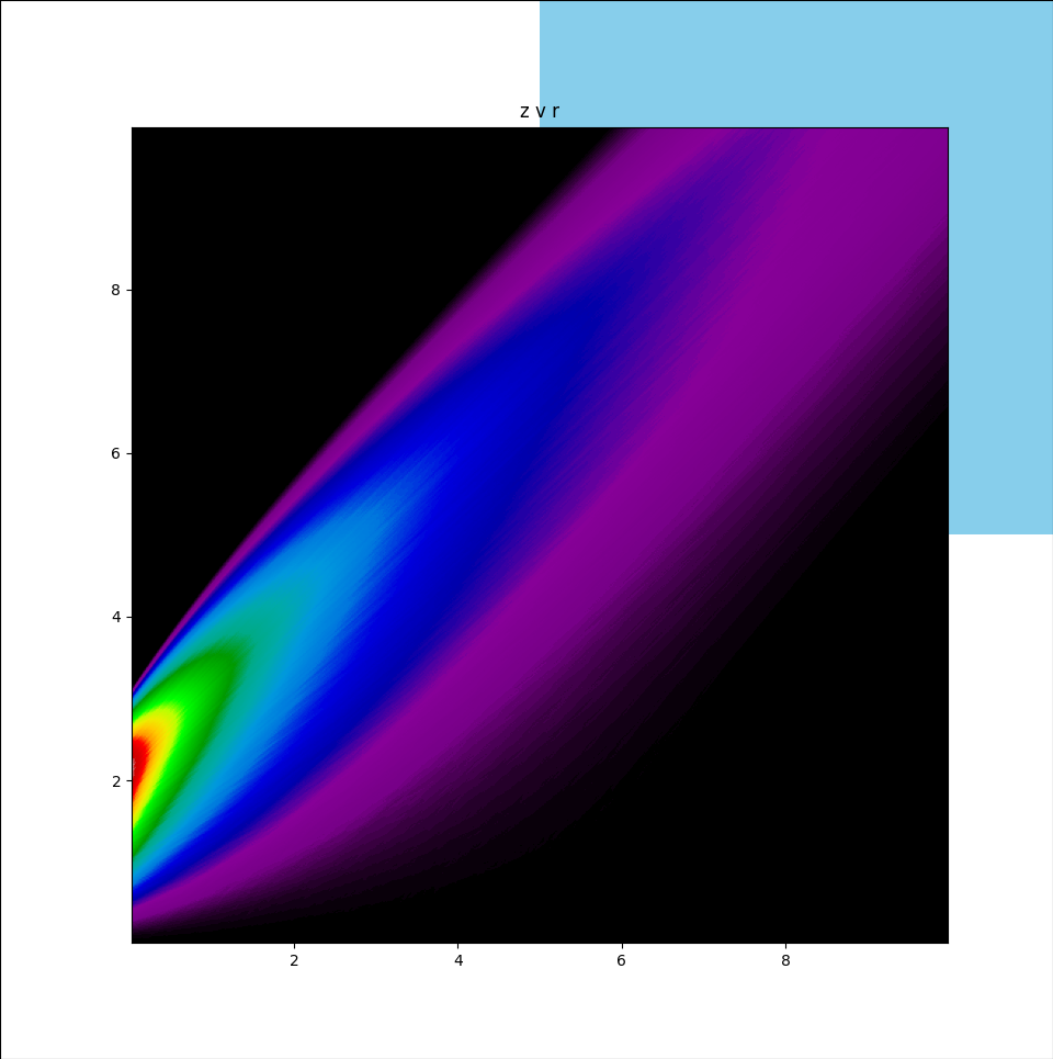
To get a better feel for the redshift distance relationship in de Sitter Space, I made a modification to the Spiral Galaxies, no dark matter module, specifically to the code that creates plots of z v r, redshift against distance, for a random sample of galaxies in de Sitter space.
The modification maps z to zdash = z / (1+z), if z < 0, zdash = z if z>=0
The idea here is that z=-1 corresponds to an infinite blue shift, so this modification stretches the values less than zero out in the same way that it stretches out in the same way redshift tends to infinity.
I have been experimenting with different windows of zdash.
Here is what a -10,10 zdash window looks like:
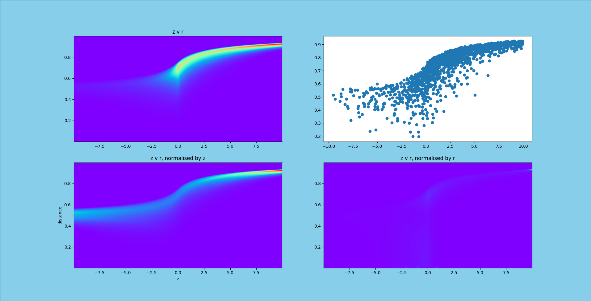
I am calling this a t-rex plot.
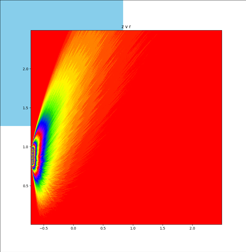
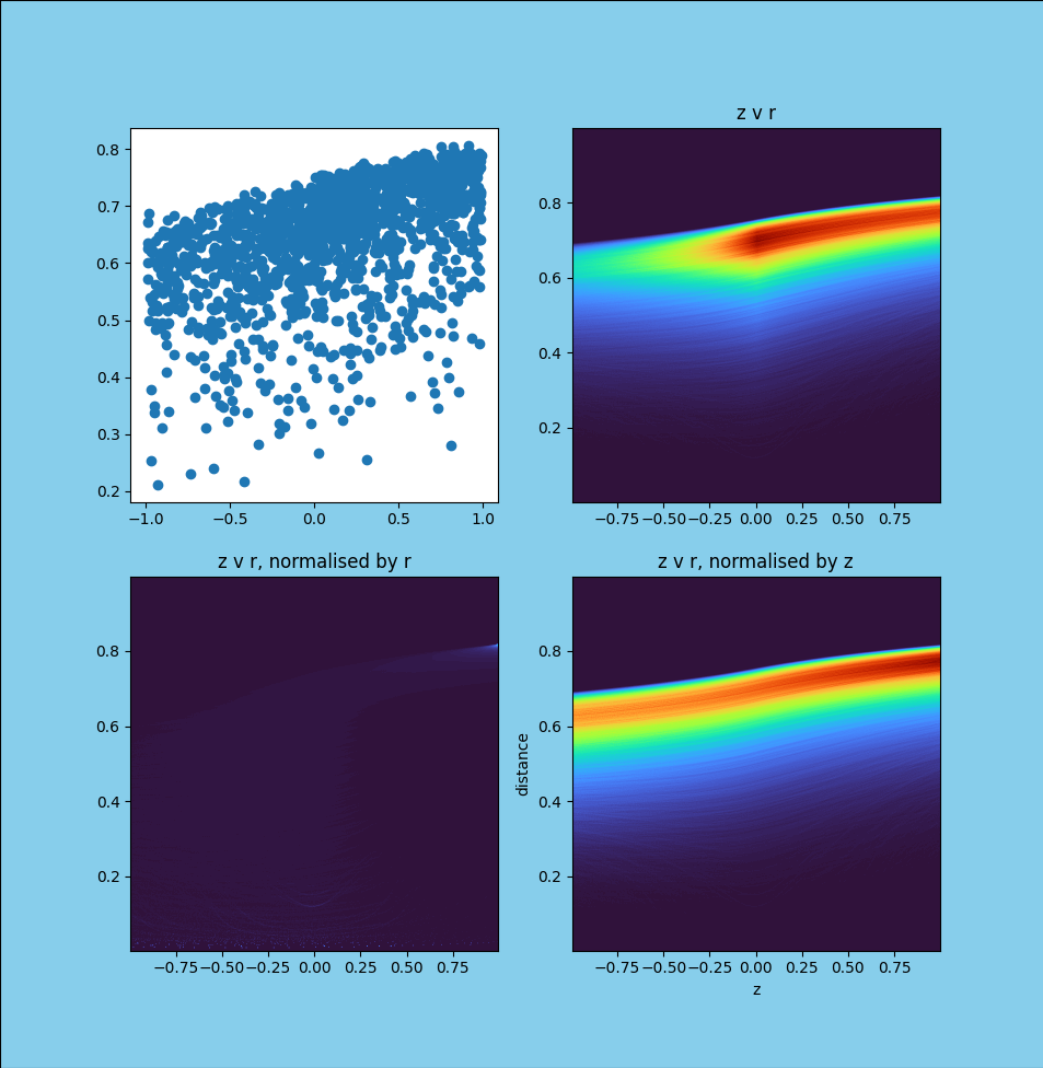
Zooming in to a smaller range of redshift, such as mod(zdash) < 0.22, we see that the picture can look very different.
It then becomes very apparent why there is Hubble tension, the image can look very different based on which range of redshifts and distances you look at.
Here is the image for abs(zdash) < 1.
One bit remaining to be modelled is the visibility, or apparent magnitude of each source. In particular, there needs to be a factor of 1/(z*z) applied to the magnitude to account for reduction in power resulting from redshift. The energy of each photon is proportional to its frequency, as are the number arriving per unit time, resulting in a reduction of 1/(z*z) in the magnitude of a source.
The pieces are coming together to model the green valley.
2025/2/1
The Fortune object here is now at the point of creating interesting pictures.
It is also at the point of showing that things are of course a little more complicated.
There is other factors that needs a model: gravitational redshift and cosmological blueshift too.
As always all this is covered in The Geometry of the Universe.
There is a quasar-galaxy spectrum, defined by the size of the object’s central black hole.
These black holes, grow slowly accreting matter over time, so larger black holes may well be much older. The gotu.spiral.Spiral module has all the key pieces, it is just necessary to put the puzzle together.
Quasars typically exhibit gravitational redshift.
The Eddington sphere, is the place where the outward radiation pressure matches the inward gravitational pull. gotu.Spiral.eddington. The radius of this sphere can be calculated, given the redshift.
If we know the mass of the black hole and the temperature and density of the medium then we can calculate z, and hence the Eddington radius.
The density must lie somewhere between the density of the black hole and the interstellar density. The latter is between 100/cm3 and 1e12/cm3.
Reasonable to assume it is lower or equal to the density of the black hole.
What is needed here is a full model for quasars evolving into galaxies.
Some general observations:
Small quasars have gravitational redshift, the Eddington sphere is close to the Schwartzchild radius.
Stars typically form further out from the Eddington sphere and hence are subject to reduced redshift.
de Sitter Space exhibits blue shift as well as redshift. We may be seeing the dust of some galaxies and mistaking it for stars.
If we assume that all redshift is cosmological, then the result is that the stars around small quasars will appear blue-shifted.
6/3/2025
Simulations of de Sitter Space show that redshift is only a weak indicator of distance, or rather asymptotically an indicator of distance.
This applies to blueshift too, where, the higher the blueshift, the closer the source is to the Hubble radius. As with redshift, this is only an asymptotic relationship.
The glowing dust of a high blueshift source may be mistaken for a redshifted view of the stars in a galaxy.
Perhaps the green valley is in part due to whether we are seeing the dust or the stars of a galaxy?
This is one area the JWST can contribute significantly. Observations of nearby galaxies at different wavelengths should help us refine our classifications of galaxies.
24/3/2025
There is a new release of data from the Dark Energy Spectrographic Instrument (DESI).
Observations are classified in various categories.
ELG, LRG, BGS, QSO
Emission Line Galaxy
Luminous Red Galaxy
Bright Galaxy Survey
Quasar Stellar Objects
DESI data release 2
It is going to be very interesting to explore the DESI data sets with the perspective of the Geometry of the Universe.
The central idea is that as the size of the central black hole grows, so does the ratio of the radius of the Eddington sphere to the Schwartzchild radius.
So small quasars exhibit significant redshift. Some of the luminous red galaxies are likely nearby quasars.
When the light comes from the accretion disk it is harder to extract a detailed spectrum, in short spectral lines are blurred.
See gotu.desi for tools to download DESI data.
2/5/25
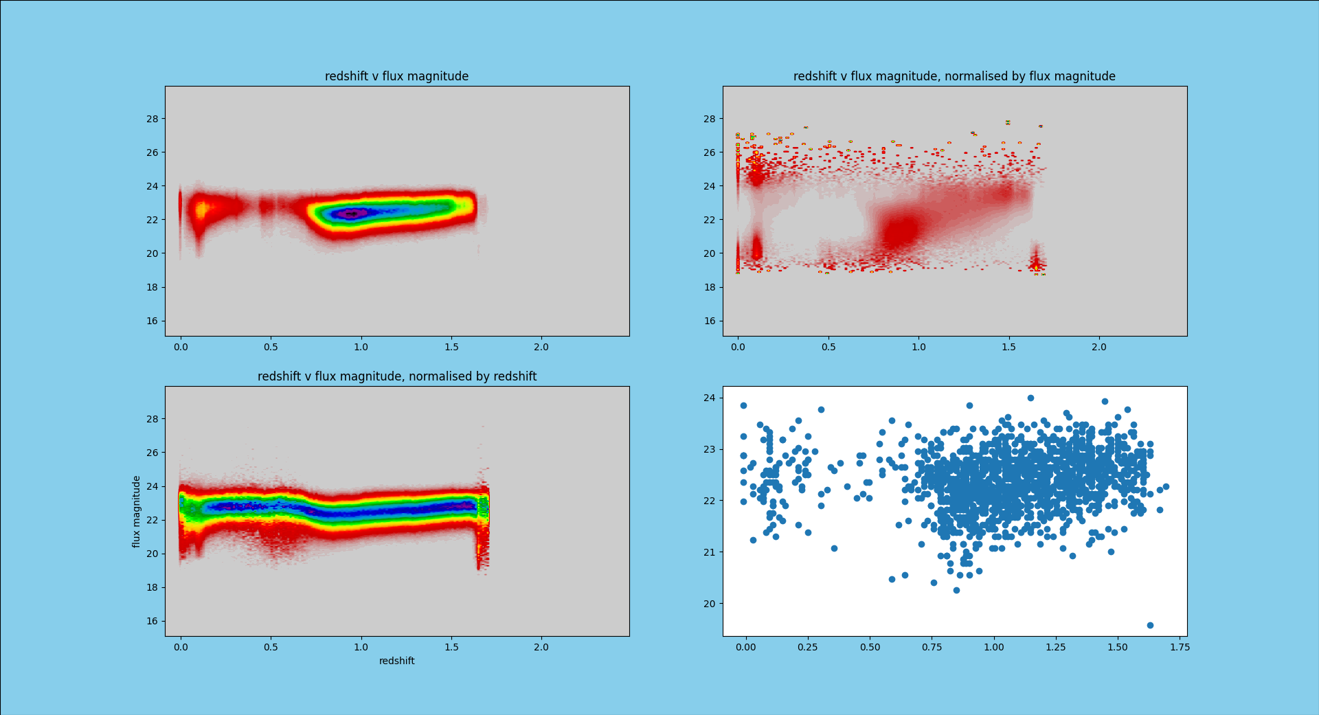
I have been using the View object here to explore the DESI data, in particular the distribution of observations by redshift and magnitude.
The DESI data release 1 paper has been invaluable in understanding the data set: https://arxiv.org/abs/2503.14745
The pictures produced are fascinating.
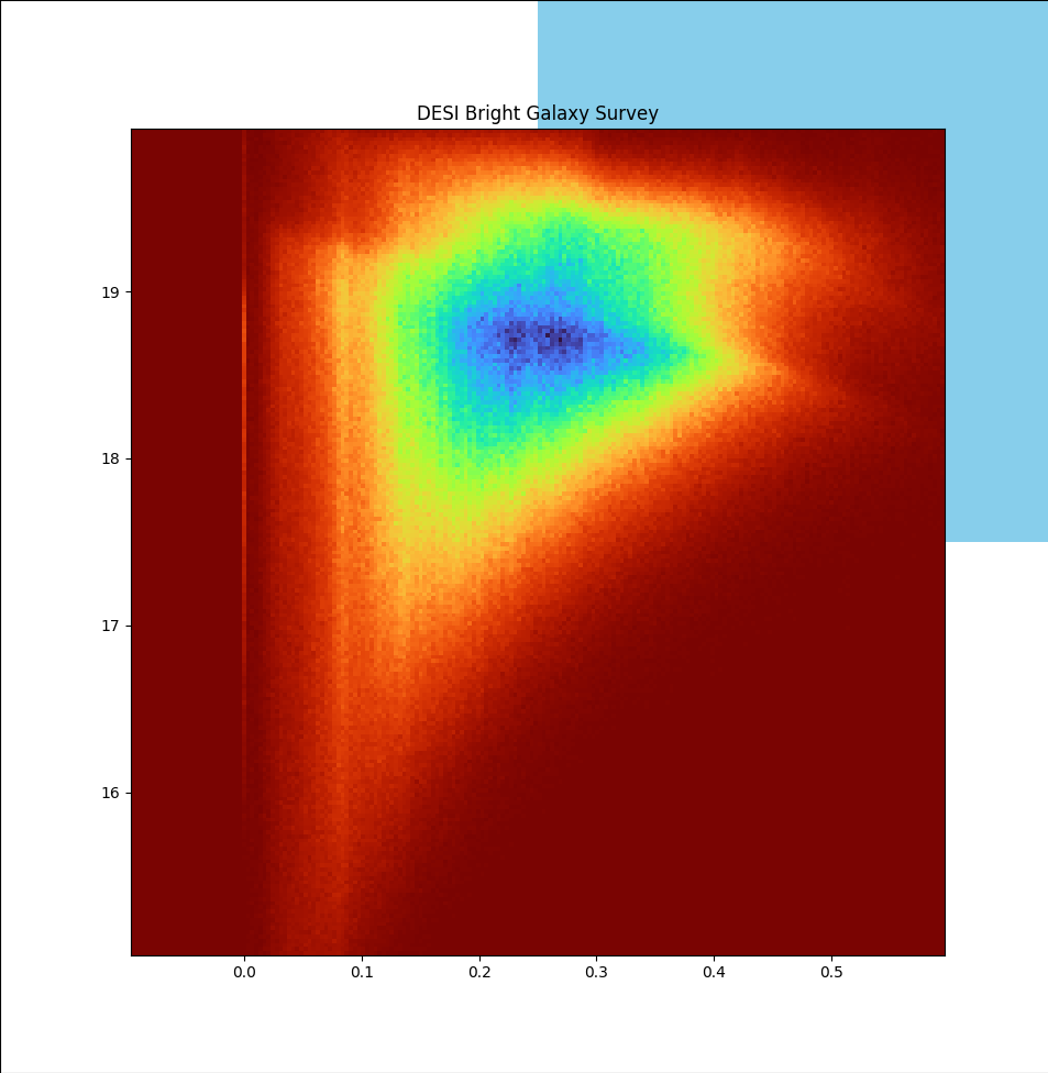
x-axis is the redshift, y-axis magnitude (FLUX_Z).
Zooming out, and including Luminous Red Galaxies, we get this image:
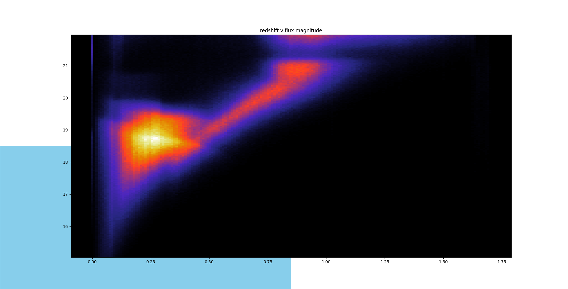
Here we see the green valley from another angle. Most of the galaxies we see are either bright (=blue) and near, or more distant and red.
There appears to have been a transition and there do not seem to be many in-between galaxies.
There is another curiosity. The DESI also includes emission line galaxies. These are galaxies for which emission lines for various elements are clearly evident.
Here is the image for emission line galaxies:
The curiosity here is that the vast majority of emission line galaxies are lower magnitude.
Rourke’s quasar-galaxy model proposes that quasars are in fact baby galaxies and as their central black hole grows by slow accretion they become mature galaxies.
Further, the model notes that the light from the central black hole can be arbitrarily close to the black hole, giving it arbitrarily large red-shift.
The redshift at the Eddington sphere depends on the temperature and density of the medium.
If we assume that the temperature and density of the medium is similar across the galaxy spectrum, then the gravitational redshift turns out to be inversely proportional to the central mass.
Now think again about the DESI data. Figure 1, from the DESI collaboration paper on data release 1 shows a stunning image of the various layers of the visible universe:
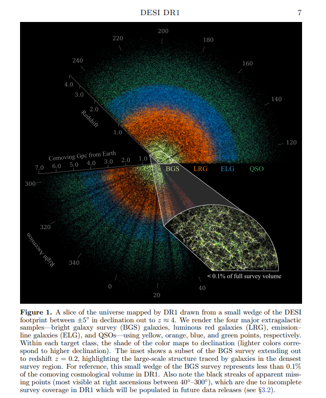
At low redshifts, we see the bright galaxies, around redshift 0.25 we move into a region of luminous red galaxies. Then we reach the emission line galaxies at redshifts 1-1.8 and finally, quasars redshifts 2-4.
Figure 7 from the same paper shows mean spectra at several redshifts: 0.2, 0.7, 1.2, 1.5 and 2.65 across this range.
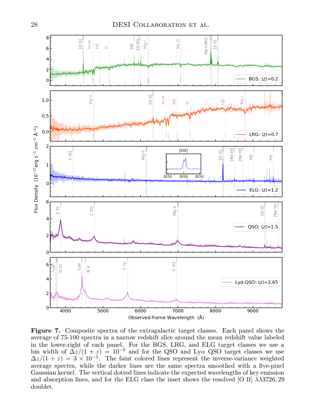
Working from the centre, with the bright galaxies, we see spectra with strong emission lines, generally not as strong and narrow as the emission line galaxies. High flux sources and low redshift.
Next, the luminous red galaxies. Emission spectra are much harder to spot and broader. Lower flux, with much of the energy at the red end.
Quasars. High redshift, with Lyman alpha forests visible for the higher redshift quasars and broad emission peaks.
Rourke argues that light from quasars has gravitational redshift and that the Lyman alpha absorption is just to hydrogen absorption by hydrogen clouds between the central black hole and ourselves.
Conventional cosmology believes the same, just that all the redshift is cosmological and the absorption is by clouds at different redshifts along the light’s very long journey to us.
In both cases, the width of the alpha forest reduces as the redshift reduces.
The amount of absorption also places constraints on the density of the medium. Too much gas and no light gets through, too little and there is not enough absorption.
Baryonic Acoustic Oscillations
Returning to quasars. DESI did some sophisticated analysis of the correlations between spectra for the Lyman-alpha forests of different quasars.
The assumption is that these quasars are very distant and that the absorption is due to clouds of hydrogen gas along the billions of light-years the light has taken to reach us.
In a big-bang model, the redshift also indicates the epoch and so the theory is that we are seeing the evolution of the density of the medium over time.
In the Rourke model, the absorption is by the surrounding gas, which is presumably concentrated in spiral arms around the central hole.
In both cases, it should be expected to have some random variation, but also correlation between objects of the same redshift.
In the Rourke model, the correlation should be between quasars with the same gravitational redshift.
It should also be noted that in the Rourke model quasars are small and of high absolute magnitude.
As such, we cannot see them beyond a certain distance.
DESI Spectra
The desi module can has tools to visualise spectra.
- class gotu.birch.Fortune[source]
- async green_valley(ball, z, x, gz=0.0)[source]
Create colour magnitude diagram
Each ball is a galaxy, redshift z and distance x.
Use self.nuvr() to calculate colour given magnitude and use self.green to make some counts.
- nuvr(mag)[source]
return nuv-r value for given magnitude
Assume a straight line relationship.
hmm.. this is wrong,
going to replace with selfcolour()
- random_mstellar()[source]
Want distribution of galaxies by stellar mass
There should be good values from local data.
The gotu.spiral module uses a lognormal distribution.
This models things well for high stellar masses, but it feels like it very much underestimates the numbers of smaller objects, below 10^9 stellar masses.
The problem here is that biggest surveys are affected by the very same problem, the assumption of an exact Hubble law.
There should however be a large enough sample of local galaxies to get a better estimate of the distribution.
- gotu.birch.apparent_magnitude(absmag, distance)[source]
Give apparent magnitude give absolute magnitude and distance
NB need distance in mega-parsecs.